The Sequential Learning Group
NeurIPS 2026
Closing the Loop: Co-Evolving EM for Irregular Time Series Generation in Lifted Representations
Gal Fadlon*, Idan Arbiv*, Omri Azencot
Irregular time-series generation is usually solved open-loop: impute once, freeze, train. We show the binding constraint is iteration, not imputer design, and close the imputer–generator loop with a co-evolving Monte Carlo EM in lifted image space.
Abstract
Authors
*equal contribution
At a Glance
Average relative improvement over the strongest baseline, across ten datasets and four corruption regimes.
Abstract
Regular time-series generation from irregular time series is typically reduced to one-shot imputation: complete each partial sequence once, freeze the completions, and train a generator on the resulting surrogate dataset. We show that this open-loop strategy is structurally flawed. Point imputers collapse ambiguous missing regions to conditional averages, while stochastic imputers become stale as the generator evolves; the binding constraint is therefore iteration, not imputer design. We introduce a co-evolving Monte Carlo EM framework that closes the imputer–generator loop. Each E-step samples missing values from the posterior of the current generator, and each M-step retrains the generator on these completions, preserving unconditional generator training. Since our diffusion prior operates in a lifted 2D representation while observations live in time-series space, we further introduce Posterior Sampling for Lifted Representations (PSLR), which enforces operator-consistent conditioning, uncertainty preservation, and manifold consistency during the E-step. Across ten datasets and four corruption regimes, our method achieves state-of-the-art performance, improving over the strongest baselines by 59% in discriminative score, 15% in predictive score, 73% in Context-FID, and 71% in feature-correlation error. Ablations show that our approach reduces average discriminative score by 73% over single-step baselines, closing most of the remaining gap to the clean-data oracle.
Key Contributions
- 1
Iteration is the binding constraint
We show, theoretically and across a 10-dataset benchmark, that closed-loop training via co-evolving EM outperforms all published open-loop baselines. Iteration, not imputer design or architectural sophistication, is the primary driver of generative fidelity under missingness.
- 2
A closed-loop framework for irregular generation
A co-evolving Monte Carlo EM that alternates between sampling missing values and retraining the generator. To make it work in lifted space we develop PSLR, a plug-and-play posterior sampler for cross-space constraints, with three structural conditions (C1–C3) any valid dual-space E-step must satisfy.
- 3
State-of-the-art on four corruption regimes
New SOTA on the standard ten-dataset benchmark, recovering near-oracle performance with rapid convergence, plus three new, harder benchmarks: per-cell asynchronous missingness, contiguous block gaps, and continuous-time irregular sampling.
Why Close the Loop?
Open-Loop Imputation Is Structurally Flawed
Prior methods (GT-GAN, KoVAE, ImagenI2R) share a commit-and-forget template: a pretrained imputer completes each irregular sequence once, the completions are frozen, and a generator is trained on them. Missing values are ambiguous, the same partial sequence admits many valid completions, but an MSE-trained imputer resolves the ambiguity by predicting the conditional mean. Across a dataset this systematically shrinks variability, so the generator learns a narrower distribution than the true one.
A better imputer does not fix this. A stochastic imputer restores diversity, but its conditional distribution is fixed before training; as the generator improves, the imputer falls out of sync. Training is unbiased only when missing values are sampled from the distribution the trained generator itself would produce, a self-referential requirement no pretrained imputer can satisfy. Closing the loop is what achieves it at every iteration.
Open loop vs. closed loop
Each E-step samples completions from the current generator's posterior; each M-step continues training from the previous weights on them.
The Conditional-Mean Trap
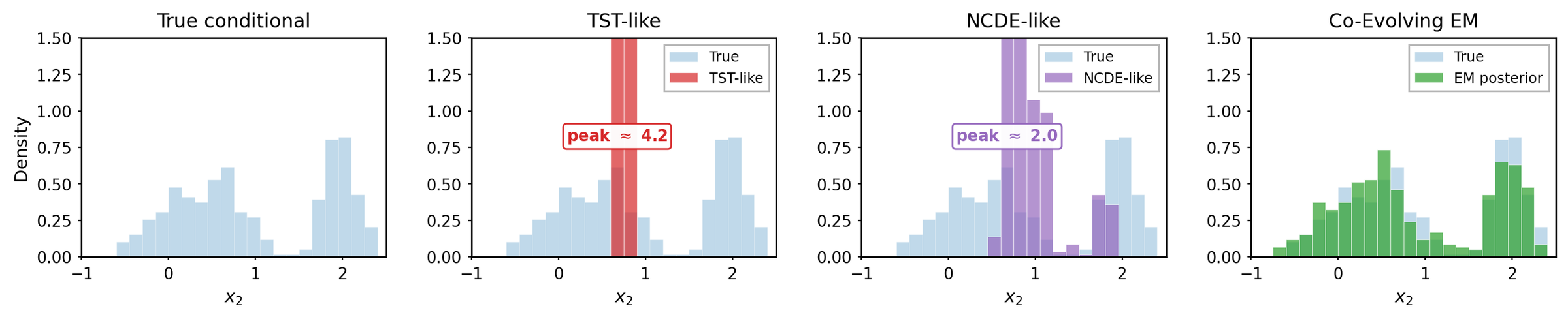
Figure 2: With a bimodal conditional p(x₂ | x₁ ≈ 0), deterministic TST-like and NCDE-like imputers collapse missing values to the conditional mean, placing mass between the true modes. Co-evolving EM samples from the current generator's posterior and recovers both modes.
The binding constraint is iteration: imputations must be refined repeatedly using feedback from the generator they are used to train.
Lower Imputation Error ≠ Better Generation
A controlled 2D experiment where the true distribution is known: two interleaved spirals, with each coordinate removed with probability 0.6. The method with the lowest imputation MSE produces the worst samples, collapsing the spirals into a regression-line cross. Co-evolving EM has almost twice the MSE yet recovers both arms.

Figure: Generated samples on two spirals at 60% missingness. Only co-evolving EM (right) recovers both spiral arms.
| Method | Imputation MSE ↓ | Generation (disc.) ↓ |
|---|---|---|
| Point regression | 2.22 | 0.390 |
| Point imputer (NCDE) | 2.46 | 0.252 |
| EM, 1 iteration | 3.65 | 0.222 |
| Frozen stochastic | 4.31 | 0.154 |
| Co-evolving EM (Ours) | 4.26 | 0.049 |
Table: Point-estimate metrics reward averaging; the downstream generation score reverses the ranking. The distributional Energy Score agrees with generation quality (Ours: 0.79, best). The same ordering holds in 21/21 configurations of a 7-distribution × 3-missing-rate sweep.
Method
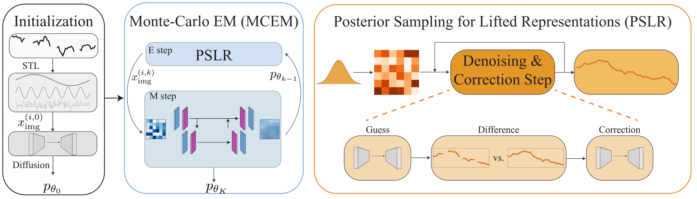
Figure 3: We initialize a generator from a simple decomposition of the irregular series, then refine it with a co-evolving Monte Carlo EM loop that alternates between posterior sampling (E-step) and generator updates (M-step). PSLR enables conditioning in the lifted space by iteratively denoising and correcting samples to match the observations.
Co-Evolving Monte Carlo EM
Each irregular series yts is a partial view of an unobserved complete series. Maximizing the data likelihood directly is intractable, so we alternate two steps on a diffusion generator that operates on lifted 2D (image) representations ximg = T(xts):
E-step: sample, don't average
Draw completions from the posterior of the current generator, so they stay consistent with what the model has learned so far.
M-step: plain training
Identical to clean-data ImagenTime/EDM training: no masked loss, no auxiliary imputation head, no separate conditional model.
Posterior Sampling in Two Spaces
The prior lives in image space, but observations constrain the decoded time series. The correct observation model is therefore the composed operator
Existing diffusion posterior samplers (DPS, ΠGDM, DiffPIR, TMPD, MMPS) assume a single space. Used as-is, they correct with the wrong operator, average over modes in ambiguous regions, and drift off the manifold of valid lifted images. PSLR (Posterior Sampling for Lifted Representations) is a minimal, sampler-agnostic recipe that enforces three conditions:
Operator-consistent conditioning
Enforce observations through the composed operator G = Ats ∘ T⁻¹ (mask after decoding the image back to a series), not an image-space mask approximation, so updates follow the true forward model.
Uncertainty preservation
Keep the full Tweedie covariance instead of a point estimate or heuristic diagonal, with an adaptive observation-noise scale σy = c·σt, so ambiguous regions stay multimodal instead of being averaged.
Manifold consistency
Project every sample back onto Range(T) via Π(x) = T(T⁻¹(x)), removing off-manifold components that would otherwise accumulate across EM iterations.
We instantiate PSLR on MMPS (full Jacobian Tweedie covariance via conjugate gradient), giving L-MMPS; applying the same recipe to TMPD gives L-TMPD, which transfers without retuning.
Full Algorithm
- 1
Init
Complete each irregular series with a cheap STL decomposition, lift it to an image, and train an initial prior pθ0 with the standard EDM objective.
- 2
E-stepfor k = 1 … K
With θk−1 frozen, sample complete lifted series ximg ~ pθ(ximg | yts) using PSLR with G = Ats ∘ T⁻¹.
- 3
Projectfor k = 1 … K
Project onto valid images, ximg ← T(T⁻¹(ximg)), and enforce the observed entries.
- 4
M-stepfor k = 1 … K
Continue training θk from the previous weights (40 epochs) on the refreshed completions, using plain clean-data EDM training.
- 5
Inference
Sample ximg ~ pθK unconditionally with standard EDM and return T⁻¹(ximg).
Modular by Design
Results
Four Corruption Regimes
All prior work evaluates a single corruption pattern. Real sensors fail for continuous periods, channels fail asynchronously, and sampling clocks are rarely uniform, so we add three new benchmarks alongside the standard one. Models are trained only on corrupted observations and evaluated by comparing unconditional samples to the fully observed data, against TimeGAN-Δt, GT-GAN, KoVAE, and ImagenI2R.
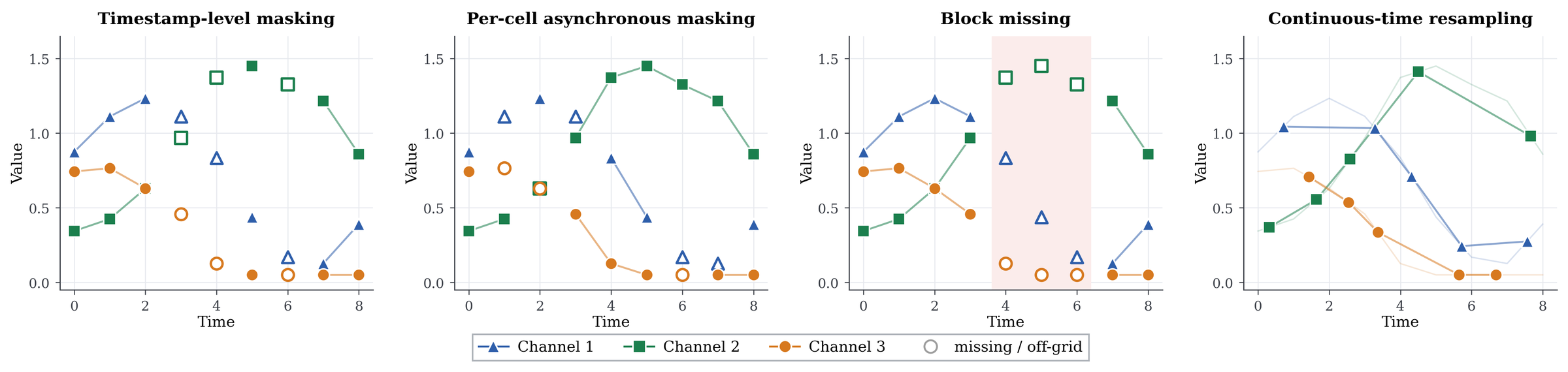
Figure 1: Four corruption regimes, all covered by a single observation operator Ats. Filled/hollow markers denote observed/missing entries.
Timestamp-level
The standard benchmark: all channels drop together at 30/50/70% of timesteps. 10 datasets × lengths 24, 96, 768.
Block missing
Contiguous gaps from sensor outages, at the start, a random location, or the end of a window.
Per-cell
Each sensor fails independently, so channels are missing asynchronously.
Continuous-time
Each channel is sampled at irregular real-valued times, off the regular grid.
Averaged Results Across Benchmarks
| Setting | TimeGAN-Δt | GT-GAN | KoVAE | ImagenI2R | Ours |
|---|---|---|---|---|---|
| Timestep (Standard) | 0.496 | 0.387 | 0.228 | 0.067 | 0.055 ↓ 18% |
| Block | 0.499 | 0.432 | 0.321 | 0.366 | 0.097 ↓ 70% |
| Per-cell | 0.494 | 0.447 | 0.341 | 0.304 | 0.116 ↓ 62% |
| Continuous | 0.498 | 0.427 | 0.326 | 0.274 | 0.043 ↓ 84% |
Table 1: Discriminative Score averaged across datasets for each corruption regime (lower is better). The percentage under our score is the relative improvement over the strongest baseline in each row. Our method is best in every setting and metric; prior methods, built around open-loop imputation, break down on the three new benchmarks.
Per-Dataset Results Explorer
Step 1: Choose Corruption Regime
A fraction of timesteps is dropped; all features at a dropped timestep go missing together.
Step 2: Choose Missing Rate
Step 3: Choose Metric to View
Currently viewing: Standard (timestamp) · Length 24 · 50% missing · Discriminative Score
| Model | ETTh1 | ETTh2 | ETTm1 | ETTm2 | Weather | Electricity | Energy | Sine | Stock | Mujoco |
|---|---|---|---|---|---|---|---|---|---|---|
| TimeGAN-Δt | 0.499 | 0.499 | 0.499 | 0.499 | 0.499 | 0.498 | 0.479 | 0.496 | 0.487 | 0.483 |
| GT-GAN | 0.462 | 0.371 | 0.407 | 0.376 | 0.496 | 0.391 | 0.317 | 0.372 | 0.265 | 0.270 |
| KoVAE | 0.188 | 0.086 | 0.057 | 0.077 | 0.498 | 0.499 | 0.298 | 0.030 | 0.092 | 0.117 |
| ImagenI2R | 0.032 | 0.005 | 0.013 | 0.013 | 0.035 | 0.360 | 0.065 | 0.014 | 0.007 | 0.007 |
| Ours | 0.011 | 0.007 | 0.019 | 0.016 | 0.020 | 0.350 | 0.042 | 0.015 | 0.009 | 0.019 |
| Clean-data oracle | 0.006 | 0.006 | 0.002 | 0.003 | 0.003 | 0.005 | 0.009 | 0.007 | 0.007 | 0.022 |
Lower is better for all metrics; the best model per dataset is highlighted. Scroll the table sideways to see every dataset. Values for our method are the minimum across the EM training history. The clean-data oracle is trained on fully observed data and serves as a reference.
Qualitative Evaluation
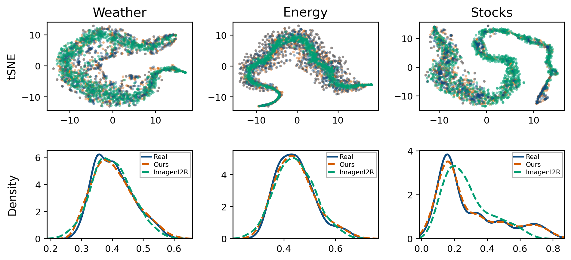
Figure: 2D t-SNE embeddings (top) and probability densities (bottom) at 70% missingness on Weather, Energy and Stocks. Our samples (orange) overlap the real data (blue) almost perfectly, while ImagenI2R (green) is more concentrated and slightly biased. Ours also wins every cell of the Wasserstein-distance comparison at 30%, 50% and 70%.
Ablation Study
A stochastic imputer (CSDI) halves the error of a deterministic one, and a single round of posterior sampling with extended training performs about the same. Neither is enough. Only iterating closes the gap, and a naive single-space sampler in the loop is not enough either: every PSLR condition contributes.
| Method | Energy | Weather | Stock | Avg. |
|---|---|---|---|---|
| Open loop: does stochasticity or more training suffice? | ||||
Point imputer (NCDE) + ImagenTime open loopdeterministicPSLR ✗ | 0.225 | 0.281 | 0.149 | 0.218 |
CSDI + ImagenTime open loopstochasticPSLR ✗ | 0.120 | 0.095 | 0.070 | 0.095 |
Ours (1 iter, extended training) open loopposteriorPSLR ✓ | 0.140 | 0.120 | 0.085 | 0.115 |
| Closed loop: does each PSLR condition matter? | ||||
Lifted-mask MMPS-EM closed loopposteriorPSLR ✗ | 0.095 | 0.098 | 0.096 | 0.087 |
w/o C1 closed loopposteriorPSLR partial | 0.065 | 0.035 | 0.014 | 0.038 |
w/o C2 closed loopposteriorPSLR partial | 0.072 | 0.048 | 0.022 | 0.047 |
w/o C3 closed loopposteriorPSLR partial | 0.078 | 0.061 | 0.031 | 0.056 |
| Full method | ||||
Ours (Full PSLR-EM) closed loopposteriorPSLR ✓ | 0.051 | 0.022 | 0.007 | 0.027 |
Clean-data oracle | 0.009 | 0.003 | 0.007 | 0.006 |
Table 2: Average discriminative score (lower is better) across Energy, Weather and Stock at 30%, 50% and 70% drop rates.
Fast Convergence
EM sounds expensive, but in practice it converges in about 5 iterations: the STL warm start begins close to the data manifold, and each M-step continues from the previous weights for only 40 epochs. Time-to-best is 58% lower than KoVAE and within 2.2× of ImagenI2R.
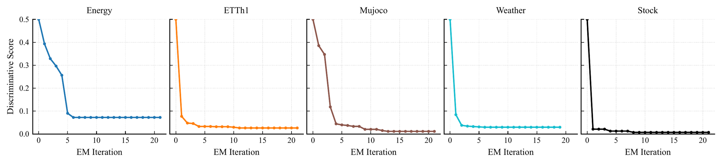
Figure: Running-minimum discriminative score per EM iteration at 70% missingness (the hardest setting). Curves drop sharply in the first few iterations and plateau within 5–13 iterations.
Wall-clock time to best discriminative score (hours, RTX 3090)
Table: Averaged across ten datasets at length 24, including all EM iterations needed to reach the best score.
Cite Us
BibTeX Citation
@inproceedings{fadlon2026closingtheloop,
  title={Closing the Loop: Co-Evolving EM for Irregular Time Series Generation in Lifted Representations},
  author={Gal Fadlon and Idan Arbiv and Omri Azencot},
  booktitle={Advances in Neural Information Processing Systems (NeurIPS)},
  year={2026}
}